40 add data labels to chart excel
Adding Data Labels To An Excel Chart | MyExcelOnline In our example below, I add a Data Label to a column chart and then I format the data label using CTRL+1. I then select to custom format the numbers so it shows the values as thousands by adding a comma , after each zero and then showing the work k by adding "k" Example Custom Number Format: [$$-1004]#,##0 ,"k" ;- [$$-1004]#,##0 ,"k" peltiertech.com › shaded-quadrant-excel-xy-scatterShaded Quadrant Background for Excel XY Scatter Chart Aug 28, 2013 · A client has a problem with a quadrant-type chart (mixed XY-Area type) in Excel 2010. This is a chart sheet, not an embedded chart. When the chart is updated, the date axis breaks. Interesting that if the chart is copied, the copy has a working date axis, and the original can be deleted. I don’t know if this helps at all.
How to add data labels from different column in an Excel chart? Right click the data series in the chart, and select Add Data Labels > Add Data Labels from the context menu to add data labels. 2. Click any data label to select all data labels, and then click the specified data label to select it only in the chart. 3.

Add data labels to chart excel
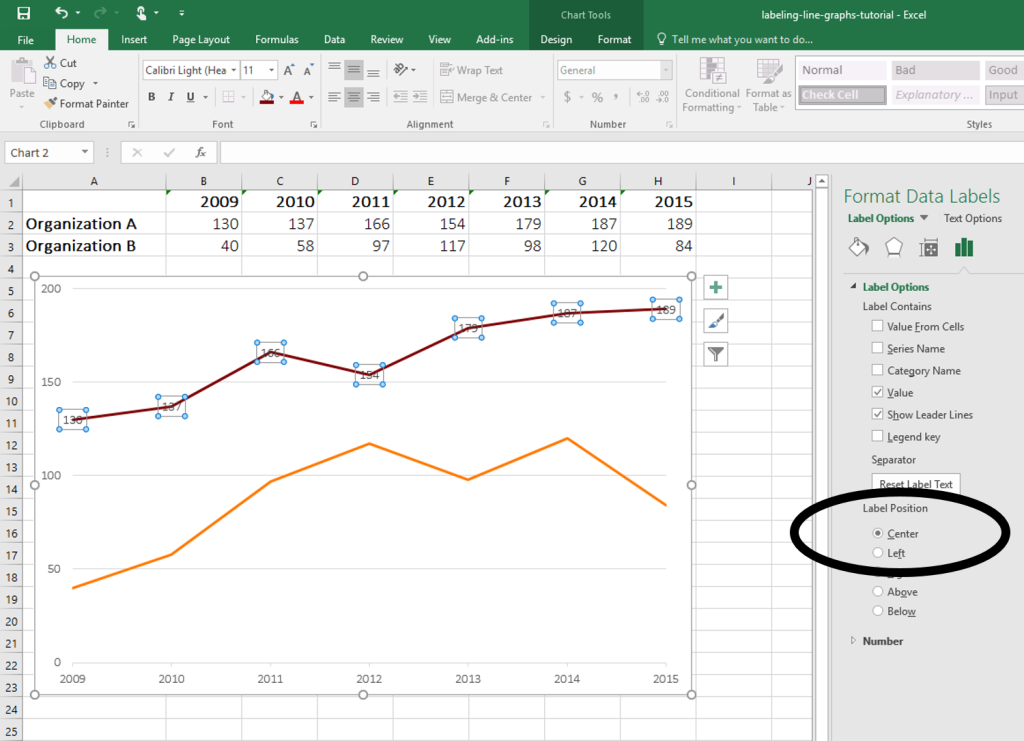
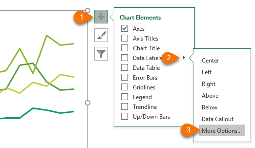
Add / Move Data Labels in Charts - Excel & Google Sheets Adding Data Labels Click on the graph Select + Sign in the top right of the graph Check Data Labels Change Position of Data Labels Click on the arrow next to Data Labels to change the position of where the labels are in relation to the bar chart Final Graph with Data Labels How to Add Two Data Labels in Excel Chart (with Easy Steps) Step 4: Format Data Labels to Show Two Data Labels. Here, I will discuss a remarkable feature of Excel charts. You can easily show two parameters in the data label. For instance, you can show the number of units as well as categories in the data label. To do so, Select the data labels. Then right-click your mouse to bring the menu. Create Dynamic Chart Data Labels with Slicers - Excel Campus You basically need to select a label series, then press the Value from Cells button in the Format Data Labels menu. Then select the range that contains the metrics for that series. Click to Enlarge Repeat this step for each series in the chart. If you are using Excel 2010 or earlier the chart will look like the following when you open the file.
Add data labels to chart excel. Apply Custom Data Labels to Charted Points - Peltier Tech First, add labels to your series, then press Ctrl+1 (numeral one) to open the Format Data Labels task pane. I've shown the task pane below floating next to the chart, but it's usually docked off to the right edge of the Excel window. Click on the new checkbox for Values From Cells, and a small dialog pops up that allows you to select a ... How To Add Data Labels In Excel - dark-team.info To get there, after adding your data labels, select the data label to format, and then click chart elements > data labels > more options. After picking the series, click the data point you want to label. Source: temotips.blogspot.com. Using excel chart element button to add axis labels. Click the chart to show the chart elements button. How To Add Data Labels In Excel - tequis.info Click on the arrow next to data labels to change the position of where the labels are in relation to the bar chart. Add A Label (Form Control) Click Developer, Click Insert, And Then Click Label. You can now configure the label as required — select the content of. To format data labels in excel, choose the set of data labels to format. › documents › excelHow to hide zero data labels in chart in Excel? - ExtendOffice 1. Right click at one of the data labels, and select Format Data Labels from the context menu. See screenshot: 2. In the Format Data Labels dialog, Click Number in left pane, then select Custom from the Category list box, and type #"" into the Format Code text box, and click Add button to add it to Type list box. See screenshot: 3.
Custom Chart Data Labels In Excel With Formulas - How To Excel At Excel Follow the steps below to create the custom data labels. Select the chart label you want to change. In the formula-bar hit = (equals), select the cell reference containing your chart label's data. In this case, the first label is in cell E2. Finally, repeat for all your chart laebls. How to Use Cell Values for Excel Chart Labels - How-To Geek Select the chart, choose the "Chart Elements" option, click the "Data Labels" arrow, and then "More Options." Uncheck the "Value" box and check the "Value From Cells" box. Select cells C2:C6 to use for the data label range and then click the "OK" button. The values from these cells are now used for the chart data labels. support.microsoft.com › en-us › officeAdd or remove data labels in a chart - support.microsoft.com Depending on what you want to highlight on a chart, you can add labels to one series, all the series (the whole chart), or one data point. Add data labels. You can add data labels to show the data point values from the Excel sheet in the chart. This step applies to Word for Mac only: On the View menu, click Print Layout. › excel-chart-verticalExcel Chart Vertical Axis Text Labels • My Online Training Hub Apr 14, 2015 · To turn on the secondary vertical axis select the chart: Excel 2010: Chart Tools: Layout Tab > Axes > Secondary Vertical Axis > Show default axis. Excel 2013: Chart Tools: Design Tab > Add Chart Element > Axes > Secondary Vertical. Now your chart should look something like this with an axis on every side:
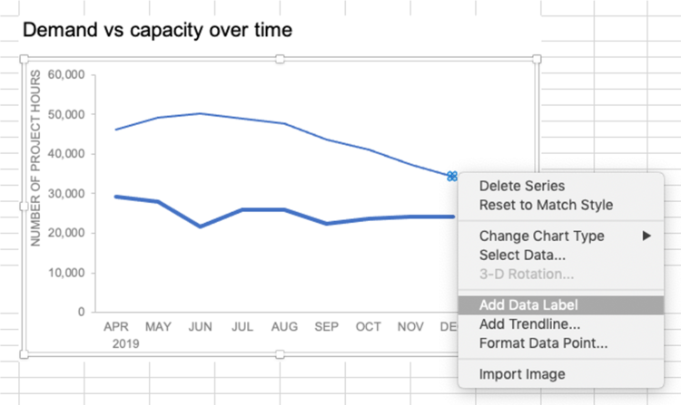
Excel charts: add title, customize chart axis, legend and data labels Click the Chart Elements button, and select the Data Labels option. For example, this is how we can add labels to one of the data series in our Excel chart: For specific chart types, such as pie chart, you can also choose the labels location. For this, click the arrow next to Data Labels, and choose the option you want. how to add data labels into Excel graphs - storytelling with data You can download the corresponding Excel file to follow along with these steps: Right-click on a point and choose Add Data Label. You can choose any point to add a label—I'm strategically choosing the endpoint because that's where a label would best align with my design. Excel defaults to labeling the numeric value, as shown below. How To Add Data Labels In Excel - militarymuseums.info Then click the chart elements, and check data labels, then you can click the arrow to choose an option about the data labels in the sub menu. Click the chart to show the chart elements button. Source: . Click add chart element chart elements button > data labels in the upper right corner, close to the chart. Click any data label ... Adding rich data labels to charts in Excel 2013 | Microsoft 365 Blog To add a data label in a shape, select the data point of interest, then right-click it to pull up the context menu. Click Add Data Label, then click Add Data Callout . The result is that your data label will appear in a graphical callout. In this case, the category Thr for the particular data label is automatically added to the callout too.
Custom data labels in a chart
Adding Data Labels to Your Chart (Microsoft Excel) To add data labels in Excel 2013 or later versions, follow these steps: Activate the chart by clicking on it, if necessary. Make sure the Design tab of the ribbon is displayed. (This will appear when the chart is selected.) Click the Add Chart Element drop-down list. Select the Data Labels tool.

Improve your X Y Scatter Chart with custom data labels
How To Add Data Labels In Excel - brzezinka.info To get there, after adding your data labels, select the data label to format, and then click chart elements > data labels > more options. After picking the series, click the data point you want to label. Source: temotips.blogspot.com. Using excel chart element button to add axis labels. Click the chart to show the chart elements button.

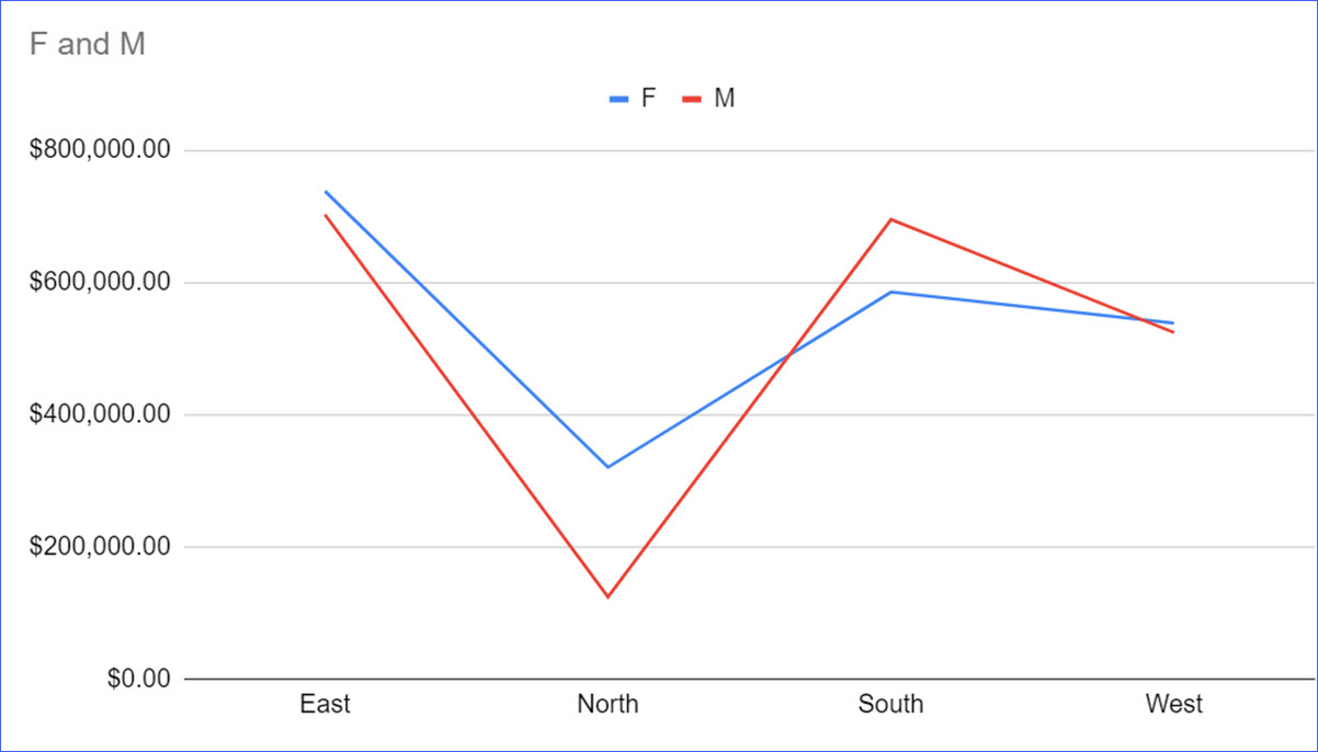
How to Place Labels Directly Through Your Line Graph in ...
Adding Data Labels to Charts/Graphs in Excel - AdvantEdge Training ... First Method - In the Design tab of the Chart Tools contextual tab, go to the Chart Layouts group on the far left side of the ribbon, and click Add Chart Element. In the drop-down menu, hover on Data Labels. This will cause a second drop-down menu to appear. Choose Outside End for now and note how it adds labels to the end of each pie portion.

How to Add and Remove Chart Elements in Excel
Add a DATA LABEL to ONE POINT on a chart in Excel Click on the chart line to add the data point to. All the data points will be highlighted. Click again on the single point that you want to add a data label to. Right-click and select ' Add data label ' This is the key step! Right-click again on the data point itself (not the label) and select ' Format data label '.

Custom Data Labels with Colors and Symbols in Excel Charts ...
Adding Data Labels to Your Chart (Microsoft Excel) - ExcelTips (ribbon) To add data labels in Excel 2013 or later versions, follow these steps: Activate the chart by clicking on it, if necessary. Make sure the Design tab of the ribbon is displayed. (This will appear when the chart is selected.) Click the Add Chart Element drop-down list. Select the Data Labels tool.

Apply Custom Data Labels to Charted Points - Peltier Tech
How to Add Data Labels in Excel - Excelchat | Excelchat After inserting a chart in Excel 2010 and earlier versions we need to do the followings to add data labels to the chart; Click inside the chart area to display the Chart Tools. Figure 2. Chart Tools Click on Layout tab of the Chart Tools. In Labels group, click on Data Labels and select the position to add labels to the chart. Figure 3.

Add or remove data labels in a chart
How to create Custom Data Labels in Excel Charts - Efficiency 365 Create the chart as usual. Add default data labels. Click on each unwanted label (using slow double click) and delete it. Select each item where you want the custom label one at a time. Press F2 to move focus to the Formula editing box. Type the equal to sign. Now click on the cell which contains the appropriate label.

how to add data labels into Excel graphs — storytelling with data
Add data labels and callouts to charts in Excel 365 - EasyTweaks.com The steps that I will share in this guide apply to Excel 2021 / 2019 / 2016. Step #1: After generating the chart in Excel, right-click anywhere within the chart and select Add labels . Note that you can also select the very handy option of Adding data Callouts.
How to Add Data Labels to Charts in Google Sheets - ExcelNotes
How to Add Data Labels to Scatter Plot in Excel (2 Easy Ways) - ExcelDemy From the drop-down list, select Data Labels. After that, click on More Data Label Options from the choices. By our previous action, a task pane named Format Data Labels opens. Firstly, click on the Label Options icon. In the Label Options, check the box of Value From Cells.
How to Place Labels Directly Through Your Line Graph in ...
Change the format of data labels in a chart To get there, after adding your data labels, select the data label to format, and then click Chart Elements > Data Labels > More Options. To go to the appropriate area, click one of the four icons ( Fill & Line, Effects, Size & Properties ( Layout & Properties in Outlook or Word), or Label Options) shown here.

Add a Data Callout Label to Charts in Excel 2013 – Software ...
How to Add Data Labels to an Excel 2010 Chart - dummies Select where you want the data label to be placed. Data labels added to a chart with a placement of Outside End. On the Chart Tools Layout tab, click Data Labels→More Data Label Options. The Format Data Labels dialog box appears.

microsoft excel - Adding data label only to the last value ...
How to add or move data labels in Excel chart? - ExtendOffice To add or move data labels in a chart, you can do as below steps: In Excel 2013 or 2016. 1. Click the chart to show the Chart Elements button . 2. Then click the Chart Elements, and check Data Labels, then you can click the arrow to choose an option about the data labels in the sub menu. See screenshot:
How to Add Data Labels in Excel (2 Handy Ways) - ExcelDemy
How To Add Data Labels In Excel - vseti.info To get there, after adding your data labels, select the data label to format, and then click chart elements > data labels > more options. After picking the series, click the data point you want to label. Source: temotips.blogspot.com. Using excel chart element button to add axis labels. Click the chart to show the chart elements button.

Stagger long axis labels and make one label stand out in an ...
Create Dynamic Chart Data Labels with Slicers - Excel Campus You basically need to select a label series, then press the Value from Cells button in the Format Data Labels menu. Then select the range that contains the metrics for that series. Click to Enlarge Repeat this step for each series in the chart. If you are using Excel 2010 or earlier the chart will look like the following when you open the file.

How to Add Total Data Labels to the Excel Stacked Bar Chart ...
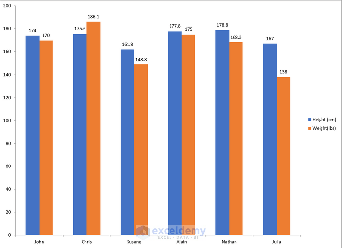
How to Add Two Data Labels in Excel Chart (with Easy Steps) Step 4: Format Data Labels to Show Two Data Labels. Here, I will discuss a remarkable feature of Excel charts. You can easily show two parameters in the data label. For instance, you can show the number of units as well as categories in the data label. To do so, Select the data labels. Then right-click your mouse to bring the menu.

Adding rich data labels to charts in Excel 2013 | Microsoft ...
Add / Move Data Labels in Charts - Excel & Google Sheets Adding Data Labels Click on the graph Select + Sign in the top right of the graph Check Data Labels Change Position of Data Labels Click on the arrow next to Data Labels to change the position of where the labels are in relation to the bar chart Final Graph with Data Labels

How to add data labels from different column in an Excel chart?
How do i add Data labels on the Pareto Line for the Pareto ...

Enable or Disable Excel Data Labels at the click of a button ...
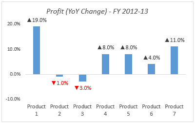
Color Negative Chart Data Labels in Red with downward arrow

How to Change Excel Chart Data Labels to Custom Values?

How to Add Data Labels to your Excel Chart in Excel 2013

Change the format of data labels in a chart

How to add data labels from different column in an Excel chart?

EXCEL Charts: Column, Bar, Pie and Line

Add or remove data labels in a chart
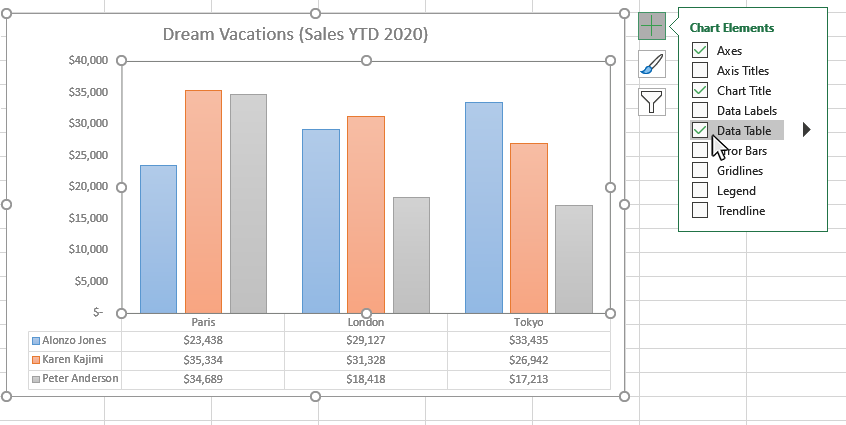
How to Add Data Tables to a Chart in Excel - Business ...

How to Add Two Data Labels in Excel Chart (with Easy Steps ...

How to add axis titles in excel chart | WPS Office Academy

Add Total Values for Stacked Column and Stacked Bar Charts in ...

Enable or Disable Excel Data Labels at the click of a button ...

Apply Custom Data Labels to Charted Points - Peltier Tech
How to Place Labels Directly Through Your Line Graph in ...

microsoft excel - Adding data label only to the last value ...
Dynamically Label Excel Chart Series Lines • My Online ...

Using the CONCAT function to create custom data labels for an ...
how to add data labels into Excel graphs — storytelling with data

Creating Pie Chart and Adding/Formatting Data Labels (Excel)

How to add or move data labels in Excel chart?

How to Show Percentage in Pie Chart in Excel? - GeeksforGeeks
Post a Comment for "40 add data labels to chart excel"